Last updated on March 1, 2022

Check the new Loss Landscape Explorer App at: https://losslandscape.com/explorer

An article published on Towardsdatascience on Medium expands this page and goes into more detail. Find the article here:
https://towardsdatascience.com/loss-landscapes-and-the-blessing-of-dimensionality-46685e28e6a4

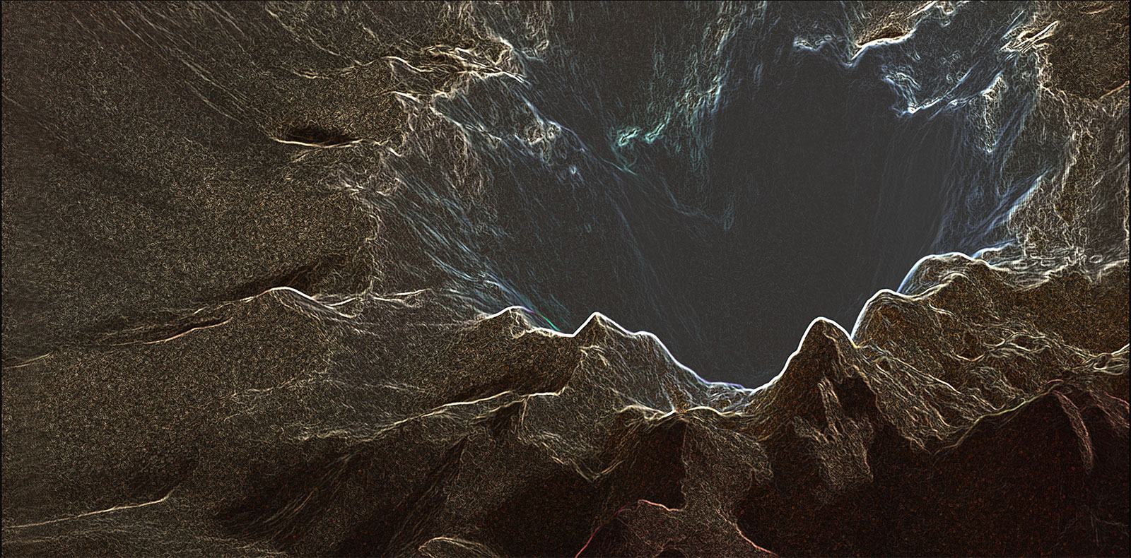
Below you can also watch some of the talks I have given about the project. Every LL piece is carefully crafted through a delicate process that combines planning, design, research, engineering and creative phases. The mission is to bring new light to the morphology and dynamics of these processes but also to inspire and challenge the viewer. This page is all about the why and the how of these representations as we ride along the minimizer and explore its nearby surroundings through the training process. Let’s go deeper into the landscapes.

• So what´s the point?

  Learning a complex function is the objective of most deep learning processes. This learning is evaluated through some kind of loss function that estimates the distance between what our network generates and what we should obtain. Minimizing that loss value is the objetive of most processes of this kind. Typically, we begin with a network that doesn’t perform very well and therefore has a high loss value. Through training, we gradually descend to loss values that are much smaller. Visualizing the morphology and dynamics of these loss values while training is taking place, can help us generate new insights about our training processes and deep learning in general.

• Can’t we do that purely through math calculations? Why do we need visualizations?

  Both are important and support and complement each other. Visualizations allow us to access simultaneously a rich amount of information that can help us jump quickly to insights that may be hard to decipher from numerical calculations.

• What are these loss values dependent on, what is the loss landscale made of?

  The loss of a network is dependent on the parameters of the network, its weights. The loss landscape is a representation of the loss values around the weight space of the network. Neural networks have typically a very large number of parameters. Therefore, the loss function is a multivariable and multidimensional function. 

• Is the loss landscape that we are visualizing a fixed shape or does it change through time?

  The shape of the landscape depends on the parameters of the network and the loss values. At each point in the training of our networks, those parameters change, and the loss values as well. As we follow our minimizer and its current weights, the visualization in a lower dimension of the surroundings of its position changes. In this sense, we can say that even though the full high dimensional landscape doesn’t change, the relative low dimensional nearby-landscape around the moving minimizer does. This low dimensional nearby-landscape becomes an ever changing dynamic system and it is through the study of its dynamics that we can gather a lot of interesting insights. It is important then to clarify that when we refer to a changing landscape, we are referring to the nearby region around the minimizer visualized in a lower dimension. This is the region we are visualizing and as the training progresses and the position of the minimizer changes, the nearby region does as well when visualized in that lower number of dimensions.

• How do we deal with so many dimensions?
  

  It is very challenging to visualize a very large number of dimensions. If we want to understand the shape of the loss landscapes, somehow we need to reduce the number of dimensions. One of the ways in which we can do that is by using a couple of random directions in space, random vectors that have the same size of our weight vectors. Those 2 random directions compose a plane. And that plane slices through the multidimensional space to reveal its structure in 2 dimensions. If we then add a 3rd vertical dimension, the loss value at each point in that plane, we can then visualize the structure of the landscape in our familar 3 dimensions. (A great reference about this strategy can be found in the excellent paper: Visualizing the Loss Landscape of Neural Nets by
  Hao Li, Zheng Xu, Gavin Taylor, Christoph Studer, Tom Goldstein)

• What about PCA?
  

  We can use the principal directions as well. However, using PCA will allow us to visualize a landscape along the most optimized directions, which tend to show the optimized parts of the landscape. Instead, we are interested in visualizing a wider range in weight space that includes other parts of the landscape that are away from our optimizer and that´s what other types of directions allow us to do.

• If the two random directions we choose make a plane that slices that high dimensional space, how can be sure that those two random directions are orthogonal to each other?

  It has been proven that in high dimensional spaces, randomly chosen vectors tend to be orthogonal to each other. You can check for the proof of this in different places online.
  
  Let’s provide a simple intuition. The more dimensions you have, the more complexity you are dealing with, and the more potential directions you can access as well. Imagine a random vector. In a 1 dimensional world, no orthogonal vector to it can exist. In a 2 dimensional world, orthogonal vectors will make a 1 D line (2-1 dimensions=n-1). In a 3 dimensional world, the orthogonal vectors will make a 2 D plane (3-1 dimension = n-1). And as you increase the number of dimensions, the possible orthogonal vectors exist in a subspace of n-1 dimensions and the larger n is, the larger share of the entire space is occupied by these potential orthogonal vectors. So, even though we cannot guarantee that two random vectors in high dimensional space will be exactly orthogonal, we can predict that they will be very nearly so.

• How do we combine these reduced dimensions?
  

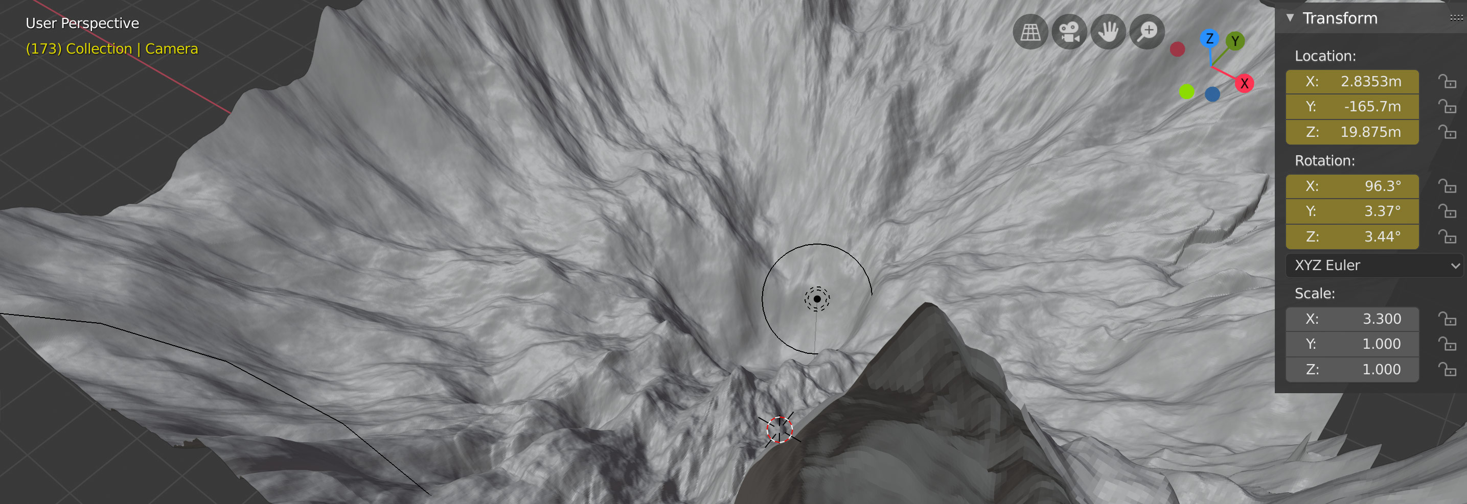
  This is one of the strategies we can use. We create a grid of points, the x and y coordinates of our representation. In the center of our grid, at the 0,0 coordinate of our landscape, we will position our optimizer. We will then explore the surrounding area around the optimizer in a certain range that we can decide. It is typical to pick the range -1,1 which is equivalent to exploring a part of the landscape of a similar magnitude to that of our weights. We can split that range (from -1 to 1) in as many discrete points as we like. A 100x100 visualization will create 100 discrete points between -1 and 1 in each of the axis. In total, we will have 10000 points to represent the landscape, and for each of those 10000 points we will calculate the loss value which will give us the vertical z coordinate of the visualization.

• How do we calculate the loss value at each of the points in the grid?

  Great question. We are going to take the weight values at the center of the grid, at our minimizer, and modify them towards the random directions we chose by an amount that depends on the point of the grid in which we are operating. Consider that:

  : represents the parameters of our network at the center of the grid, the parameters of our minimizer.
  , : they represent two random directions in weight space
  , : they represent the coordinates of one of the points in the grid.

  Then, the loss of a specific point of our visualization is the result of calculating the loss of our network using a new set of parameters born from adding the ones of our minimizer to the sum of the product of each direction by the specific coordinate we are considering.

  

  Therefore, each point in our loss landscape will have the coordinates:
  

• How do we zoom in and out our view?

  To zoom in and out, all we need to do is to change the range by which we modify our minimizer´s weights along the plane spanned by the random directions. If instead of using a -1, 1 range, you use a -0.4, 0.4 range, you will be focusing the detail of the visualization in a smaller area around the minimizer. If you use a -2, 2 range, you will be zooming out to view an area that extends further away from your minimizer.

• How far can we go?
  

  The issue here is that as you get further from the minimizer you will find that typically the loss values become really large, the landscape shoots up and no other interesting features are found. That´s why typically the interesting area we explore is in the -1 to 1 range. We also tend to use the log of the loss values when visualizing in order to contain the extreme loss values that begin appearing towards the edge of the representation.

• How can be sure that what we are visualizing provides useful information? and how precise are these visualizations?
  

  This is a great question. Transforming the very large number of dimensions of these networks into very few, immediately implies the need to be cautious and realistic. We know that we cannot be fully visualizing the enormous complexity provided by all those extra dimensions.

  Some people have pointed out that using different sets of directions may generate different kinds of landscapes. So if your objective is to get a very precise idea of the shape of the loss function, you need to be careful and cautious when analyzing these landscapes. However, the point is: can we get from this dimensionality reduction useful information? Yes indeed. And can we get the specific information we need? The answer is yes, depending on what our objective is. 

  Before we continue, let’s consider what happens when we take photographs with our mobile phones. We are transforming the 3D reality into a 2D representation. Different filters and treatments further impact and distort that “3D reality”. Our perspective, the angle from which we take the photo comes into play as well. And we could continue on and on. Let’s now face 2 questions. First, is the photograph an accurate representation of “reality”? Definitely not. But is the photograph providing useful information about that “reality”? information that can be helpful and also inspire? Definitely yes. That’s why we take photographs. And taking those photographs from different angles and perspectives, provides different insights and information which all together brings our understanding of the subject to a new level. Beyond that, we also have to consider that everything is relative, literally. Our “3D reality” is nothing more than another interpretation-distorsion produced by the human brain. We are in fact dealing with two different interpretations of the underlying “reality”, and both can provide useful information and inspire.

  A similar thing happens with the extreme dimensionality reduction and related processes when we visualize loss landscapes. Are these landscapes accurate representations of the underlying multidimensional “reality”? Surely not. But are they providing useful information about that underlying mathematical “reality”, and can that information eventually trigger new insights about the related processes? Surely yes. For example, it has been shown that the key areas of convexity and non-convexity shown by these representations match with those provided by numerical analysis performed through the main related eigenvectors and eigenvalues.

  Beyond the shape, we can focus on the dynamics of these landscapes. For example, if our objetive is to understand the change in dynamics of these landscapes as we modify different hyperparameters, we can indeed get useful information through these visualizations. 

  Therefore, surely we are not seeing the entire complexity that exists in all that large number of dimensions. And by choosing different kinds of directions we will also visualize that high dimensional surface from different perspectives (just as when we take a photograph from different angles). But the important thing is that through these visualizations we can indeed gather useful insights. And as I said above, it is particularly useful to study these landscapes in movement. In the same way that looking at a static photograph can lead to way more confusion than looking at that same scenario in motion, analyzing loss landscapes in motion help us understand much better their dynamics, behaviour and state at each of the sampled moments.

  But we don’t have to stop here. We can also use mathematics to validate these landscapes and check if, for example, the convexity distribution we observe corresponds with what numerical analysis tells us. For that, we can use the Hessian and its eigenvalues.

  The hessian matrix contains the second order derivatives and can help us understand the curvature of the loss landscape. To do that, the easiest way is to study the essence of the Hessian through its eigenvalues and eigenvectors. We know that fully convex functions have positive semi-definite Hessians with non-negative curvature values. The opposite happens with non-convex functions.

  As arXiv:1712.09913 states, the main curvatures of these simplified landscapes are weighted averages of those of the full dimensional function. Because of that, studying the eigenvalues of our landscape allows us to estimate that, on average, our visualizations are correct.

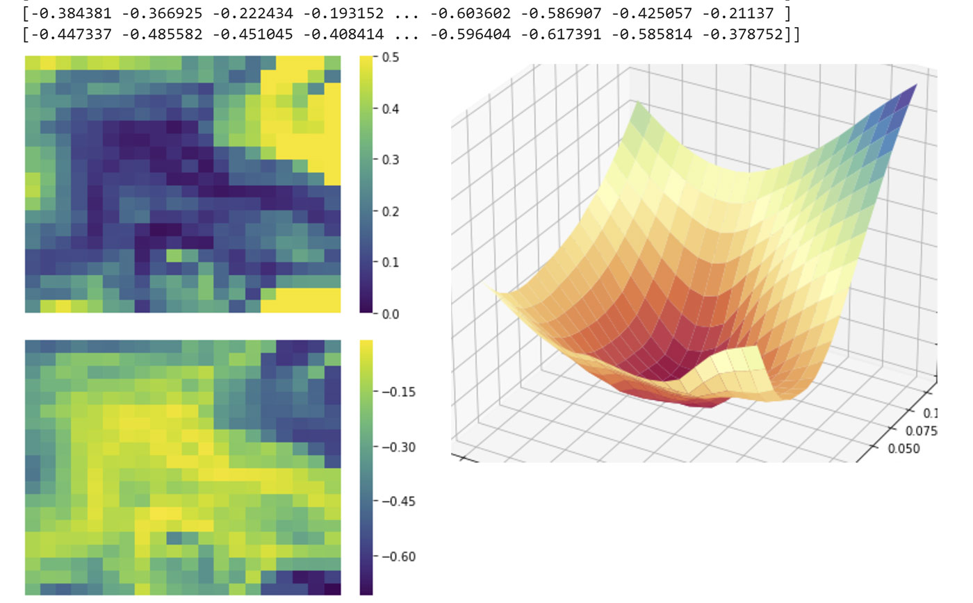
  By calculating the minimum and maximum eigenvalues of the Hessian at each point of our visualization, we can use their absolute ratio to map their distribution in order to study which areas have more or less convexity. Then, we verify that areas that look very convex in our visualization correspond to areas where negative eigenvalues are tiny. Conversely, non-convex areas in our plot correspond to areas with large negative eigenvalues.

• Why do we use eigenvalues?
  

  The Hessian matrix is a complex entity and many complex systems can be understood in better ways by working with some of their properties which are universal and capture some of their essential qualities.

  Eigenvalues and eigenvectors help us understand and capture the most essential and key features of many systems, in this case of the Hessian matrix. We capture that essential information with a series of numbers and vectors, which is simpler than having to deal with the entire and typically very large square Hessian matrix.

  Besides, these numbers and vectors give us very specific information about the properties of the Hessian matrix, which are not so easy to perceive from the full matrix representation.
  Eigenvalues and Eigenvectors are used in many different fields to extract the essence of a system. For example, they are used in image compression by discarding the small eigenvalues from the system.

• What specific information give us the eigenvalues when evaluated at a specific point?
  

  If the Hessian at a point is positive definite (all eigenvalues are >0), then we know we are looking at a local minimum of the function, therefore at a point of convexity.
  If instead, the Hessian is negative definite (all eigenvalues being <0), then we are dealing with a local maximum and a point of negative curvature). If we have a mixture of positive and negative eigenvalues, we are dealing with a saddle point instead.
  Different combinations of eigenvalues, when plotted, allow us to understand from numerical analysis the kinds of convexity patterns we have in the landscape.

• Can we extract all the eigenvalues of the Hessian Matrix?
  

  The Hessian matrix of a large neural network has a very large size, which is proportional to the square of the number of parameters of the network. Computing with the entire Hessian is not possible in any network of a significant size. Therefore, it is not practical to attempt to gather all the eigenvalues. Instead, we use the Scipy library and some algorithmic tricks to gather the smallest and largest eigenvalues and eigenvectors, which is enough for us to derive the information we need.

• Would it be feasible to keep the global loss landscape static and show a moving learner/optimizer in action? (question by -how to dowtle- @ twitter)?
  

  That’s a great question. What we are doing in these representations could be called “follow the minimizer and examine its nearby surroundings”. We can do this because we always know the state and weights of our minimizer and we can take it as center and reference point within a low dimensional plane (created from random orthogonal directions) from whose perspective we can take a look at its surroundings (nearby surroundings which constantly change because the position of the minimizer changes as well within the entire non-changing full landscape).

  Let’s now think of the alternative. The following applies to doing what the question describes with precision, not in a rough, approximate way. So, if we would like to fix in place the landscape while the training progresses and while we contemplate the path followed by the minimizer around the landscape, we have a challenge.

  The landscape we are seeing is a low dimensional interpretation of an area of the full higher dimensional one. And to create that lower dimensional representation we need a reference point, which, of course, is our minimizer. If we want to independently represent the landscape and the minimizer’s path, we are missing something crucial. What part of the higher dimensional loss landscape should we show at each stage of the process? Obviously we want to show the part near the minimizer. And we can do that. But when the minimizer moves, what should we do? How does the minimizer’s trajectory relate to the area of the landscape we are visualizing? We realize that the minimizer is not going to move within that previous lower dimensional plane. The minimizer moves within a higher dimensional structure. And the low dimensional representation of the area of the landscape where the “next” position of the minimizer will be, may have nothing to do with the previous one. If we fix the landscape, we are also fixing a low dimensional representation on a plane for a specific state of that minimizer.

  You could try to get around the issue in different ways. For example, the paper “Visualizing the Loss Landscape of Neural Nets”, uses PCA to study the optimizer´s trajectory, but the PCA directions are only going to show us the optimized parts of the landscape. And we won’t have a way to match that with precision to the rest of the landscape (a wider and more diverse area of the surrounding landscape, whatever that may be). You may take a single state, a single fixed landscape state and try to match a minimizer’s trajectory (using PCA) to it using projections, if the movement of the minimizer is very low dimensional. Still, as Tom Goldstein once told me, the minimizer’s trajectory won’t be perfectly planar so we have to project it onto a plane, and because of that, the contours projected might not be the ones that exist off the plane. PCA limits you in other ways as well in relation to the surrounding landscape. In the end, matching trajectory and landscape with precision remains an obstable, and finally, the challenge on top of the above is to do that over the entire process blending both an extensive area of the surrounding landscape and the minimizer’s trajectory.

  One of the core issues is that we are always working with low dimensional interpretations of the higher dimensional structure. Imagine taking a few photographs (lower dimension interpretation) of a subject (existing in a higher dimensional space) from different angles and then trying to match them. This is possible with Photogrammetry (https://en.wikipedia.org/wiki/Photogrammetry), which can extract the underlying 3D “reality” from a mix of 2D sources. Could we do this with loss landscapes? The challenge is that Photogrammetry makes a transition from multiple 2D sources to 3D. Instead, loss landscapes have a very high number of dimensions. Maybe, probably, in the future, there will indeed be a way of bringing this together but at the moment it remains an active area of research.

  The visualizations of this project are a way for us to join the high dimensional ride attached to the minimizer itself. While we ride along the minimizer, we use a low dimensional plane to study its surroundings from a certain perspective. If we don’t ride on the shoulders of the minimizer and instead stay in place, looking at part of the landscape from a fixed low dimensional interpretation, the minimizer will move onto a different part of a higher dimensional structure whose low dimensional representation is different. As we don’t live in and cannot see such higher dimensional structure, and as we always need to slice it somehow with a lower dimensional representation, fixing that low dimensional representation becomes possible if the movement of the minimizer happened in a very constrained number of dimensions. As this cannot be guaranteed, finding a precise way to bring together these 2 representations (minimizer’s path and fixed landscape) becomes a challenge.

  That’s why, instead, we safely ride on the shoulders of the minimizer while studying its changing surroundings as we go, which is enough to potentially provide useful information and new insights about the morphology and dynamics of these processes.

• What are some of the challenges with which loss landscape visualizations can help us?
  

  There are countless possibilities because visualization allows us to go deep into so many areas. The study of the dynamics of optimization processes is one of them. Weight pruning and subnetworks is another of the most exciting topics in which these visualizations can help us. Research is suggesting that pruning weights or training with subnetworks within our network can produce the same level of accuracy in our results while using much less time and resources. Visualizing loss landscapes can help us identify what impact has on the landscape the pruning of these weights and the use of different subnetworks.

• Can a complex function be approximated by a simpler one?
  

  The Taylor series (an expression of a function in an infinite sum of terms) is an example of how we can prune some of the complexity of a function and still retain its most essential characteristics. 

• When calculating loss landscape related values, do we have to iterate through our entire training set?
  

  If you want perfection, yes. But as usual, Pareto often beats perfection. In general, It depends on what your objective is. For certain objectives, you can iterate on a subset of the entire set as long as you are always using the same subset. As an example, the paper “Negative eigenvalues of the Hessian in deep neural networks” has verified experimentally that using 5% of the training set (repeating always the same samples in that 5%) provided results that were close enough to those that used the entire set for the purpose of analyzing the eigenvalues of the Hessian.

• Do flatter minima in loss landscapes generalize better?

  This question has received opposing opinions in the last years. The paper “Sharp Minima Can Generalize For Deep Nets” by Laurent Dinh, Razvan Pascanu, Samy Bengio, Yoshua Bengio, states that sharp minima can generalize as well as flat ones, and that flat ones can generalize poorly as well on occasions. In the paper, flatness is defined as the size of a region that has more or less constant error.
  Many other papers state a different view. Most recently, the paper “Understanding Generalization through Visualizations” demonstrates that generalization error correlates well with the flatness of the minimizer, and that differences between flat and sharp minima are emphasized by the multidimensional nature of these landscapes. This paper also concludes that high dimensionality keeps the minimizer away from bad minima.

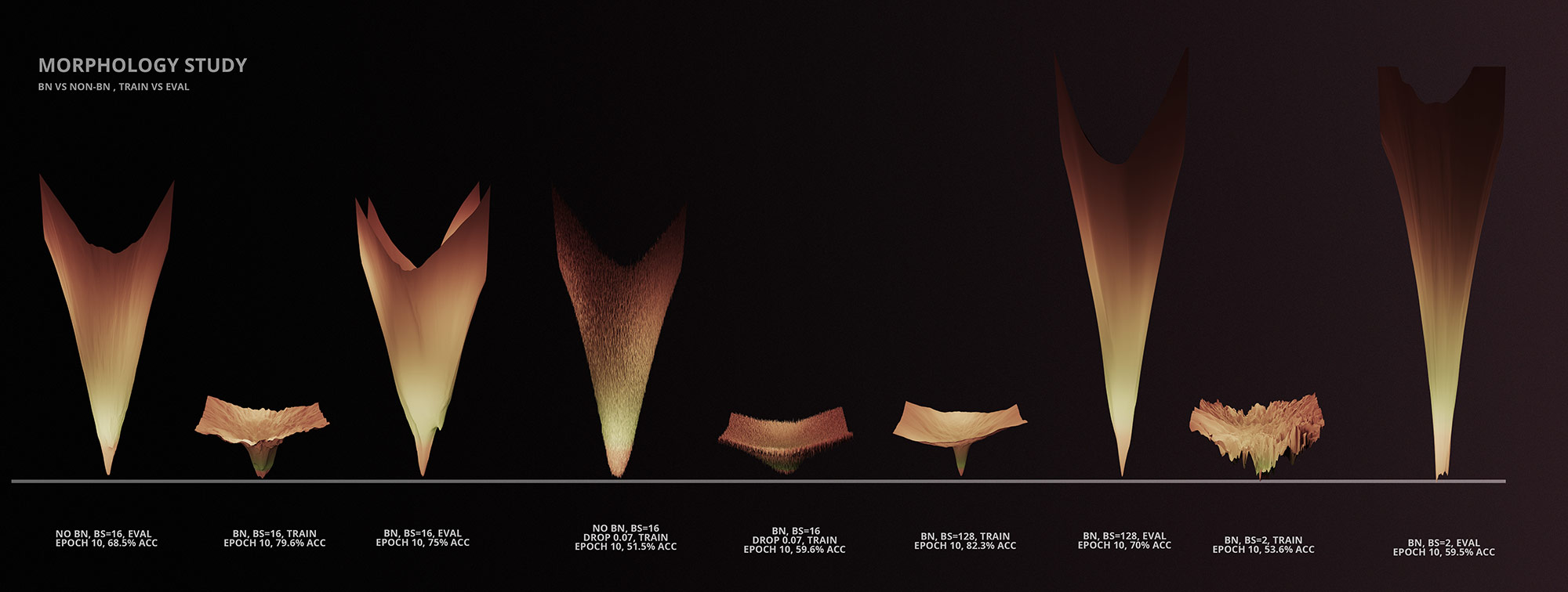
• How strong is the impact of different network parameters in the morphology of the Loss Landscape?

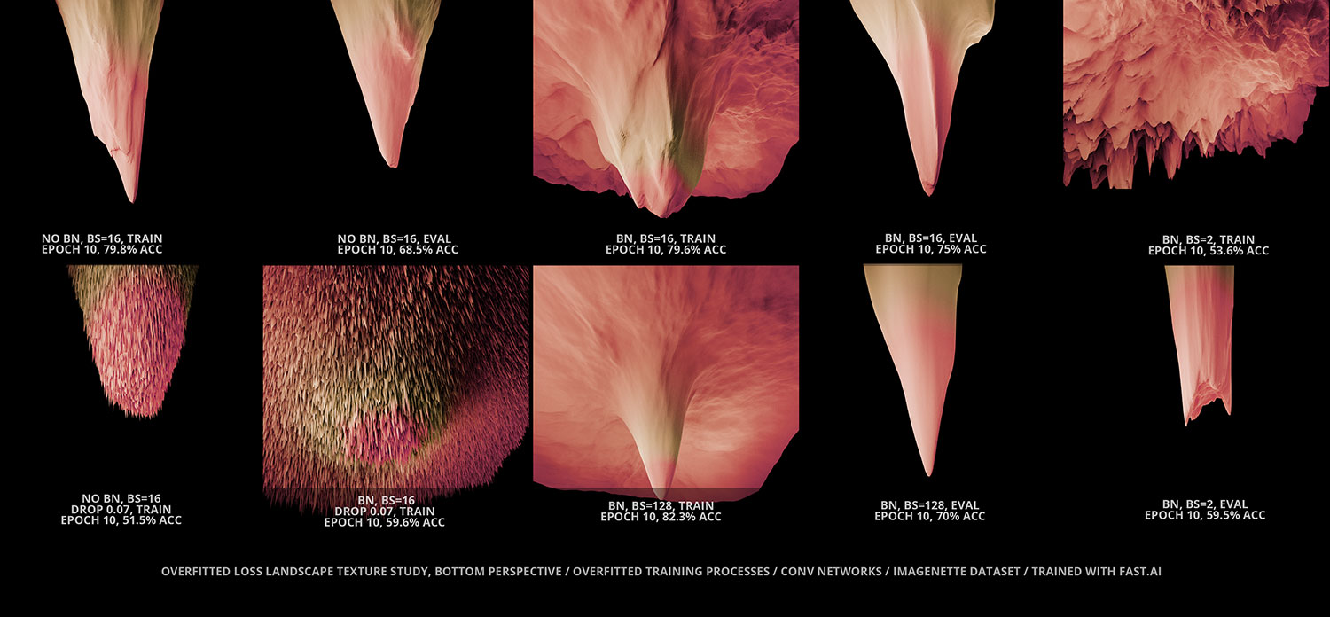
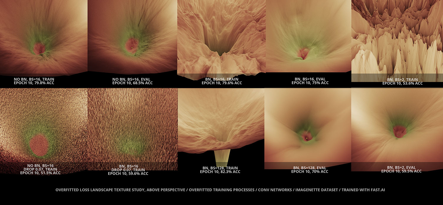
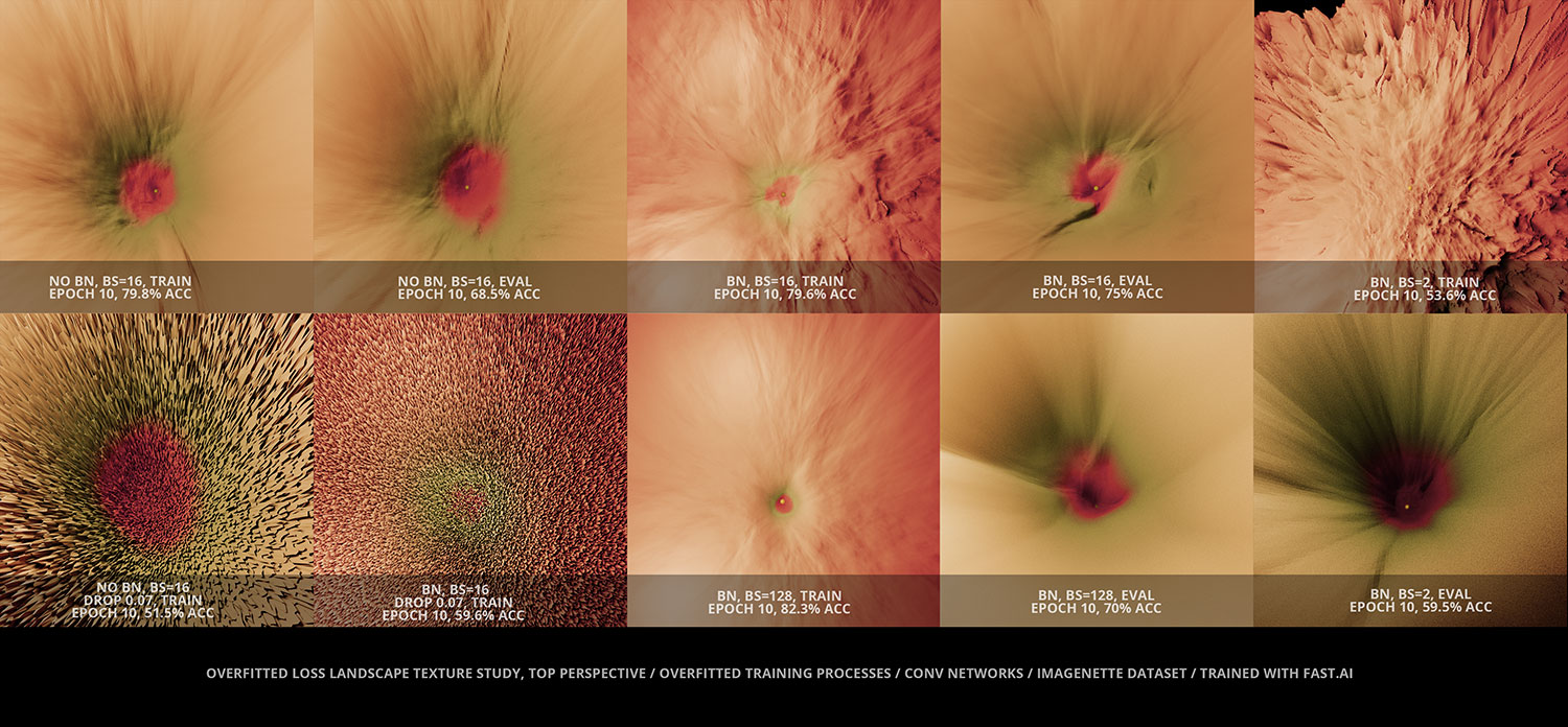
  It can be very strong during the training phase. For example, using or not using Batchnorm, or the use of dropout can have a dramatic impact in the morphology of the landscape while in training mode. More details about different insights derived from these pieces will be shared in the future through audiovisual and/or written form.

• What’s next?

  More related writings and more visualizations and audiovisual creations in the intersection of research and art, as well as collaborations with researchers around the world, going further and deeper into the fascinating world of loss landscapes. Phase 2 of the LL project is currently being prepared. Contact me on ideami@ideami.com

Gratitude

A big thank you goes to the Fast.ai community, for inspiring me constantly with their amazing spirit and knowledge, and to the team formed by Hao Li, Zheng Xu, Gavin Taylor, Christoph Studer and Tom Goldstein, authors of the paper that sparked my initial interest in the world of Loss Landscapes. Thank you for inspiring the deep learning community with your teachings, research, spirit and ventures. Thank you as well to the friends that supported me during this phase with feedback and encouragement, including David García, the hispanIA group, the Plyzer family and others.